Make a map already

We already have R, we have tools for map data, we have a crs.

This is not what we want.

plot(coast)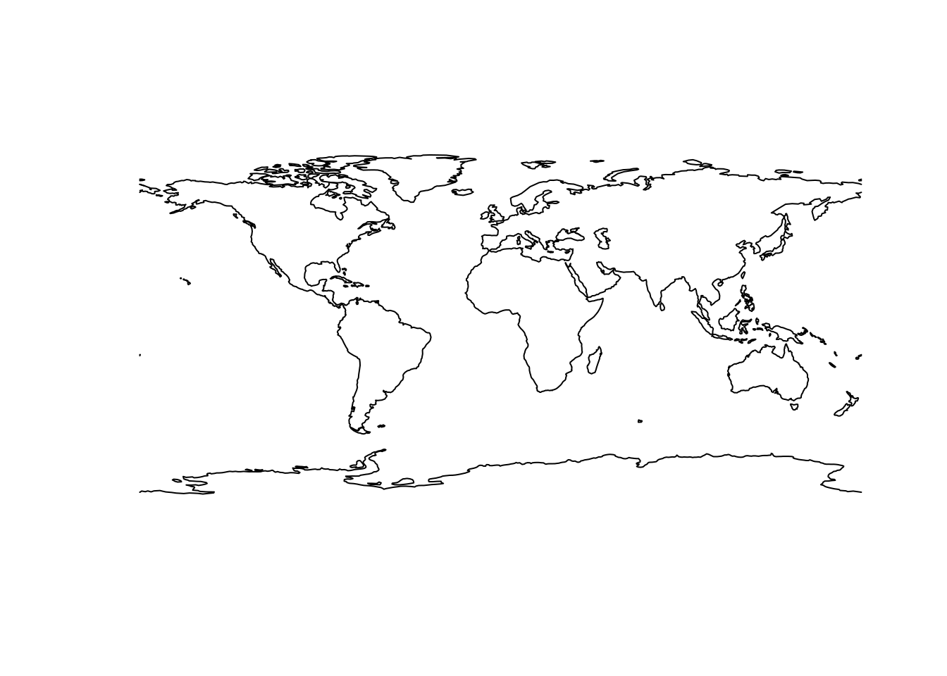

proj4string(coast)

## [1] "+proj=longlat +datum=WGS84 +no_defs +ellps=WGS84 +towgs84=0,0,0"

This map layer is “unprojected”, it uses a “longitude-latitude” coordinate system. This is not what we want but it’s absolutely critical that we (and our software) know precisely what coordinate system the data is already in.

We can transform from one coordinate system to another using sp::spTransform (this is the part where ‘rgdal’ is required, behind the scenes it does the work to interpret the ‘crs’ and transform the coordinates). The result is a replacement of the complicated Spatial object with an exactly the same complicated object with just the coordinates transformed, and the metadata updated. If anything goes wrong the process will throw and error and fail completely.

pcoast <- spTransform(coast, crs)
plot(pcoast)

Now that we have prototyped the workflow we can experiment with the projection to choose what we want.

By chaining the tasks together we can interactively see the result of choosing a new specification for the projection quickly.

crs <- CRS("+proj=laea +lat_0=-90 +lon_0=142 +datum=WGS84 +no_defs")
plot(spTransform(coast, crs))

Central longitude or latitude of the projection.

## change the lon_0 parameter, it's  rotation
crs <- CRS("+proj=laea +lat_0=-90 +lon_0=10 +datum=WGS84 +no_defs")
plot(spTransform(coast, crs))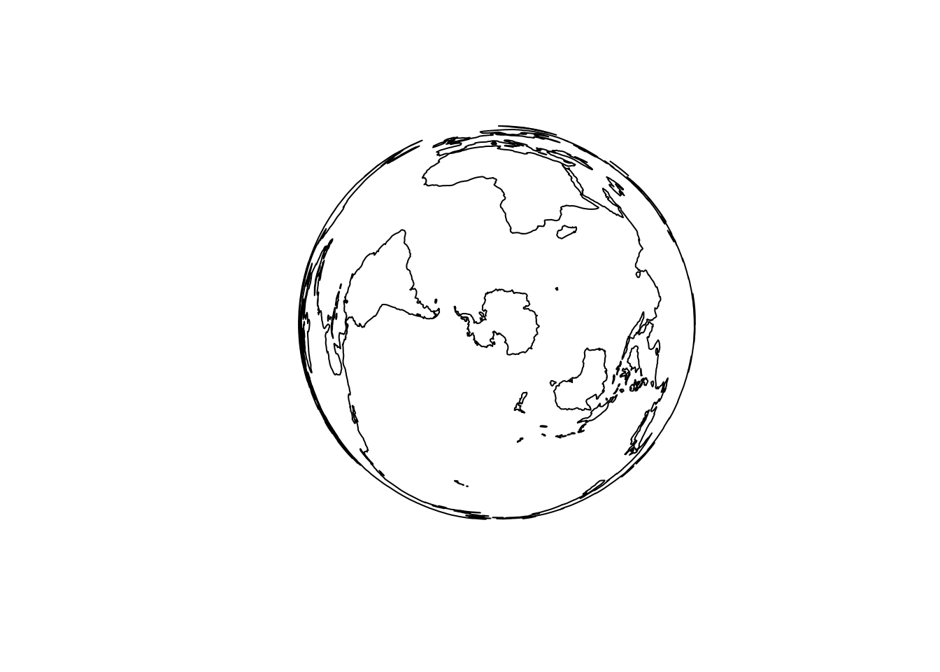

Change the datum.

## a new datum changes the relative locations
crs <- CRS("+proj=laea +lat_0=-90 +lon_0=10 +ellps=sphere")
plot(spTransform(coast, crs))
axis(1)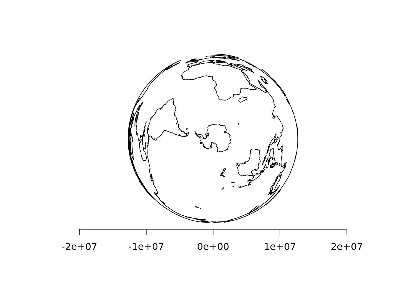

Change the family.

## a new projection family is completely different
crs <- CRS("+proj=lcca +lat_0=-90 +lon_0=10 +datum=WGS84")
plot(spTransform(coast, crs))

A projection “family” is particular choice of mathematical compromises, choose some mixed bag of area, distance, and shape. The parameters of the central longitude and latitude specify the orientation of the geographic earth with respect to that projection. Other parameters such as false eastings and northings ‘+x_0/+y_’ exist for convenience, to push the map in two directions in the plane to avoid negative numbers. Again other parameters are more substantive, they affect the orientation and detail of the surface onto which the data is projected, for example does the cone glance the globe at a tangent point or does it intersect at two latitudes (thereby reducing the “edge effect” that would other reduce the region within the magic zone of “nice conformal”).

## a new projection family is completely different
crs <- CRS("+proj=lcca +lat_0=-90 +lon_0=10 +datum=WGS84")
plot(spTransform(coast, crs))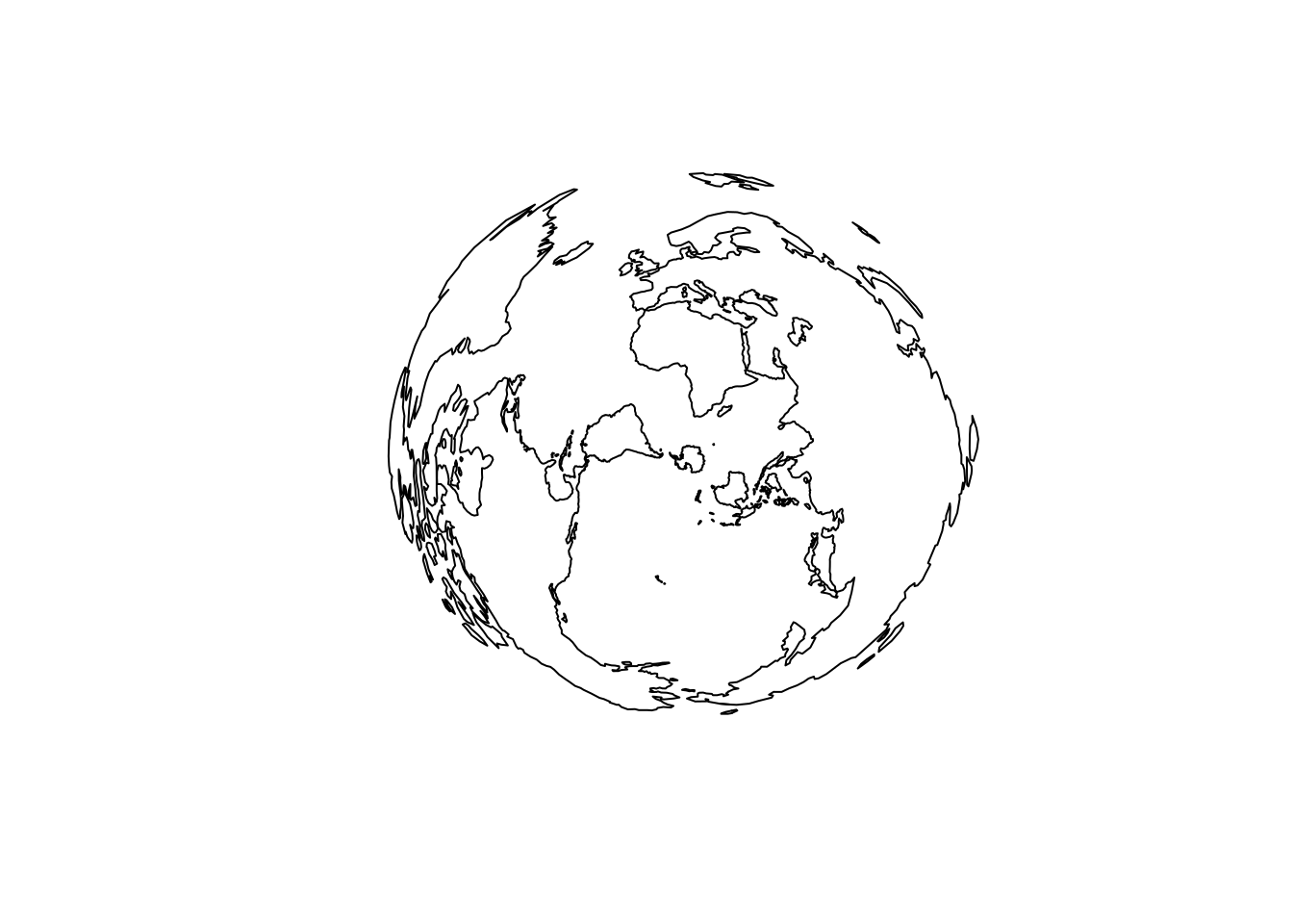

Some projection choices cause problems, though this takes us into deeper issues that we reserve for another post.

## a new projection family is completely different
crs <- CRS("+proj=ortho +lat_0=-90 +lon_0=10 +datum=WGS84")
try(spTransform(coast, crs))

## Warning in .spTransform_Line(input[[i]], to_args = to_args, from_args =
## from_args, : 12 projected point(s) not finite

## non finite transformation detected:
##            [,1]     [,2] [,3] [,4]
##  [1,] -6.197885 53.86757  Inf  Inf
##  [2,] -6.032985 53.15319  Inf  Inf
##  [3,] -6.788857 52.26012  Inf  Inf
##  [4,] -8.561617 51.66930  Inf  Inf
##  [5,] -9.977086 51.82045  Inf  Inf
##  [6,] -9.166283 52.86463  Inf  Inf
##  [7,] -9.688525 53.88136  Inf  Inf
##  [8,] -8.327987 54.66452  Inf  Inf
##  [9,] -7.572168 55.13162  Inf  Inf
## [10,] -6.733847 55.17286  Inf  Inf
## [11,] -5.661949 54.55460  Inf  Inf
## [12,] -6.197885 53.86757  Inf  Inf
## Error in .spTransform_Line(input[[i]], to_args = to_args, from_args = from_args,  : 
##   failure in Lines 2 Line 1 points 1:2:3:4:5:6:7:8:9:10:11:12

## a new projection family is completely different
crs <- CRS("+proj=merc +lat_0=-90 +lon_0=10 +datum=WGS84")
plot(spTransform(coast, crs))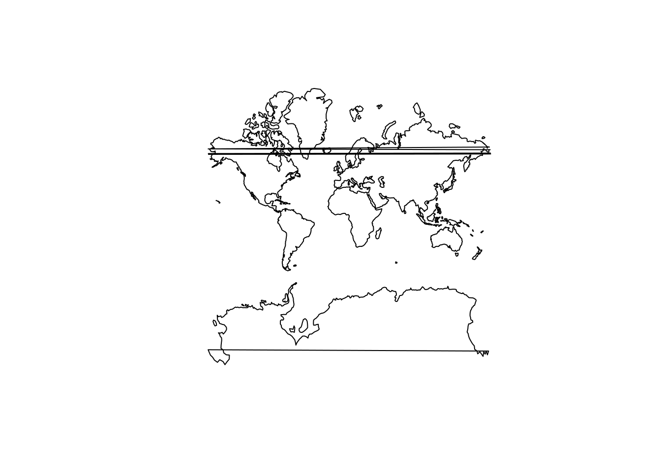

What’s next?

We have only just scratched the surface, the next steps we need might include the following.

• a local, specific, extent (this is surprisingly difficult to get right)
• a “graticule”, i.e. lines of constant longitude and latitude
• other data on the map, again this can be suprisingly complicated
• labels
• aesthetics and scales for the data on the map
• accoutrements (scale bars and north arrow and the fancy white-black margin real maps use)

Every one of these requires painstaking, back and forth experimentation and decisions. It’s just not possible to automate everything about this, so the more familiarity you have with the component tools in the process the better your maps will be. I always refer to it as “chicken-egg”, first we choose an extent or let the data define the extent of the map frame, but then we want either more or less and have to modify the initial choice or heuristic, and this then impacts subtly on other choices we had to make. You have to go back and forth a bit.

I’m kidding about the last one, for those I think it’s best to find a cartographic tool or just draw it using Microsoft Paint. I think they are pretty pointless and will end up sucking a lot of time. A scale bar is not completely accurate unless you orient it within the map in a place where linear distance on the ground correspods to equal spacing in the map (this is rare), and the north arrow is either totally redundant or hopelessly inaccurate. This is a rich are of discussion for maps, and exploring what’s wrong with north arrows, scale bars leads us into techniques for drawing graticules, reprojecting map data composed of dicsrete, straight-line segments, depicting vector fields, and calculating the Tissot Indicatrix.